Visualize imaging data

In this tutorial you will learn the basics of the DataViewer app to visualize and explore different types of imaging data. The DataViewer app open the following types of imaging data:

Images: 2D arrays with dimensions Y,X.
Image time series: 3D arrays with dimensions Y,X,T(ime).
Event-triggered image time series: 4D arrays with dimensions Y,X,T,E(vent).
Correlation Maps: 3D arrays with dimensions Y,X,S(eed).

Here, we will explore some of the data created in the previous tutorials on how to Preprocess imaging data. This tutorial focuses on the basic use of the DataViewer app to explore individual imaging dataset. To learn about all the functionalities of the app, read it's full documentation here.

Sections

Open imaging data: open imaging data in DataViewer through the main GUI or as a standalone.
Basic data exploration: explore an image time series data to learn the basics of DataViewer.
Visualize functional maps: explore a Seed-pixel correlation map.
Visualize event-triggered data: explore event-triggered image time series.

Open imaging data

You can launch DataViewer from the main GUI or as a standalone from Matlab's command window.

Launch DataViewer from the main GUI

In Matlab's command window, launch the main GUI:

        umIToolbox('C:/FOLDER/projectfile.mat');

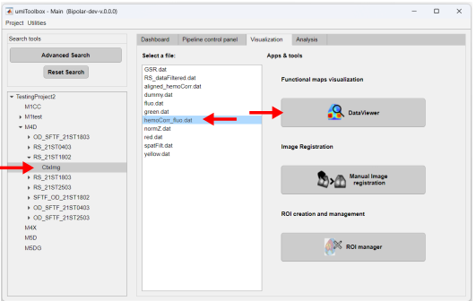
Go to the Visualization tab. Then select the object containing the file to be opened (step 1). In the Select a file: list box, select the file (step 2) - in this example, HP_tempFilt.dat. Finally, click on the app's button (step 3) to launch DataViewer:

Launch DataViewer as standalone

To open an imaging file in DataViewer directly from Matlab's command window,launch DataViewer with the full path of the file as input:

        DataViewer('C:/FOLDER/PROJECT_SAVEFOLDER/HP_tempFilt.dat');

Alternatively, launch the DataViewer app:

        DataViewer

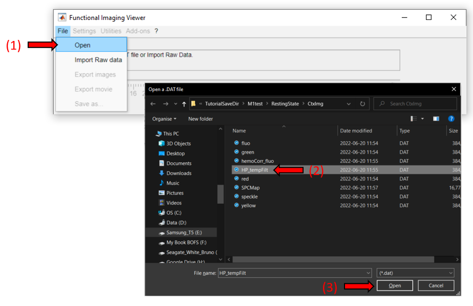
In DataViewer's main window, go to File >> Open and select the .dat file to open:

Basic data exploration

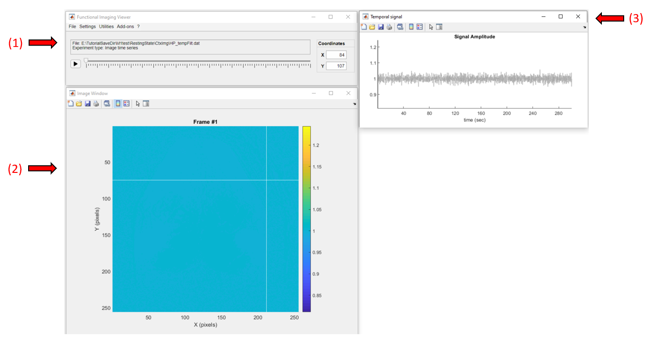
In this tutorial, we will explore an intermediate step from the preproceesing of a resting state experiment. The data stored in the file HP_tempFilt.dat consists of the fluorescence signal that was corrected for the hemodynamic artifacts, followed by the removal of the global signal variance and temporally filtered and normalized (check the tutorial on preprocessing data for resting state for details).

Below is a screenshot of the app with the data loaded. It consists of three windows: the main window (1), where all the options and controls are located, the image window (2) where the current frame of the data is shown, and the temporal signal window (3) where the temporal profile of the selected pixel is displayed.

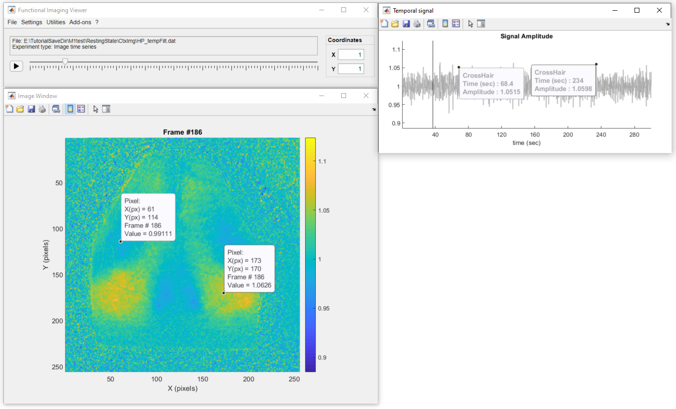
Click on a pixel to get it's temporal profile:

To change frames, either move the slider in the main window or double-click on the plot from the temporal signal window:

Also, use the figure's datatip tool tt_dataviewer_datatip_icon to add fixed data tips over the image or the temporal profile to show the pixel values as so:

Important
Don't forget to deactivate the datatip button before interacting with the figure. Some of the figure's interactions are suspended when the datatip mode is active.

Now, let's adjust the color scale limits to better visualize the fluctuations of the fluorescence signal across the mouse cortex. To do so you can simply use the vertical zoom option on the temporal signal window as so:

If you want to give a precise number, go to Settings >> Image Options and change the values of min and max. In addition, we can also change the default colormap through the Image Options:

Finally, we can use the playback button to display the "movie" of the fluorescence signal. This recording was obtained with a frame rate of 5Hz (default playback speed). We can change the playback speed in Settings >> Playback speed. Below, we can observe the fluctuations of the fluorescence signal across the mouse cortical areas (playback speed at 3 times the real frame rate):

Visualize functional maps

The functional connectivity maps created in this tutorial were stored in the file SCPMap.dat. This data consists of a 3D array containing correlation values where each frame represents the correlation map for a given seed pixel.

When visualizing a correlation map, the behaviour of the image's crosshair is different from the other imaging data types. Here, when clicking on a pixel, the correlation map is updated to show the map from the selected pixel as the seed:

Visualize event-triggered data

For images and image time series split by events, the DataViewer app shows an extra window, the Events window, containing the conditions and event repetitions. You can select one repetition or the average (#Average). The example below was drawn from the tutorial on preproceesing event-triggered data and it represents the normalized fluorescence signal of a whiskers stimulation split in 10 trials.