Create functional connectivity maps

How to create functional maps

Generating functional connectivity cortical maps

Here, we describe the steps to preprocess calcium imaging data to generate functional connectivity maps from a mouse cortex. In this example, you will learn:

How to create a pipeline to process resting-state data.
How to customize the parameters of analysis functions.
How to save, load and run pipeline files.

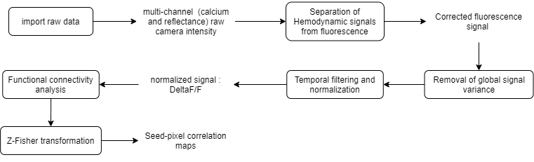
This example is a good place to start using umIT's automatic processing pipeline and its portfolio of functions given that resting-state experiments are fairly simple (a short recording of a mouse at rest).

The raw data used here consists of ~5 min multi-channel (fluorescence and reflectance) recordings of an awake mouse expressing GCaMP6 calcium indicator in cortical neurons. Here is the analysis workflow that we will create and apply to this data:

Functional connectivity pipeline workflow

Sections

Select the data: select the data to be processed.
Create and run the analysis pipeline: build the analysis pipeline to be applied to the selected data.

Select the data to be processed

Here, we assume that the project file was created. For more info on how to create a project file click here. To open a project file, call the umIToolbox app with the full path to your project file as input as:

        umIToolbox('C:/FOLDER/projectfile.mat');

Note
Here, we show how to create an analysis pipeline using umIT's main GUI. However, the same process can be applied to a single experiment using the DataViewer app as standalone. For more info on how to use DataViewer, read the app's documentation.

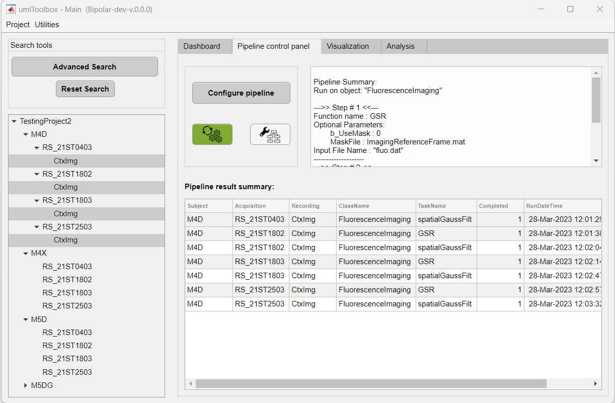
In the GUI, go to the Pipeline control panel tab:

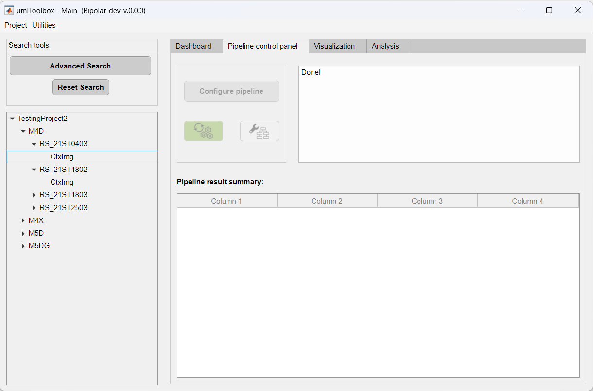
Now, we need to select the recordings to be processed. Here, you can select multiple recordings and apply the analysis pipeline to all of them. In this example, we will process all resting state recordings from the mouse M4D. In the object tree, click on the subject node to select all recordings:

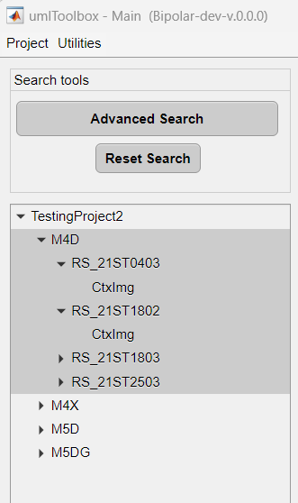
Now, the Configure pipeline button is enabled and you are ready to create the pipeline.

Create the analysis pipeline

The analysis pipeline is created using the Pipeline Configuration app. To launch the app, click on Launch Pipeline Config. A dialog box will appear so you can select which object type you want to run the pipeline. In this example, the imaging data is associated with the object FluorescenceImaging:

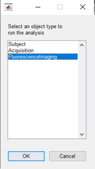
Note
This step exists only when the pipeline is run through the umIToolbox app. This step doesn't apply to data analysed using the DataViewer app as standalone.

In the Pipeline Configuration app, select the functions to generate the pipeline to create Seed-pixel correlation maps:

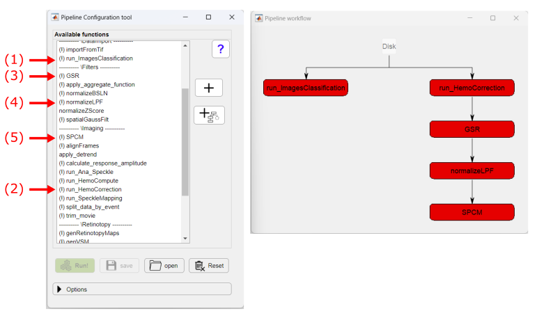
For more details on how to use the Pipeline Configuration app, click here.

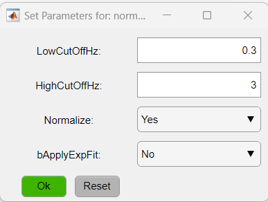
The exclamation point (!) shown before the function's name, indicate that the given function has optional parameters that can be customized. To access the parameters, click on the function's button (red buttons in the figure above). In this particular case, we will change the parameters of two functions: normalizeLPF and SPCM. For the normalizeLPF function, we will change the frequency cut-off values to filter our data between 0.3 and 3 Hz and we set the Normalize parameter to 1 to normalize the data as ΔF/F:

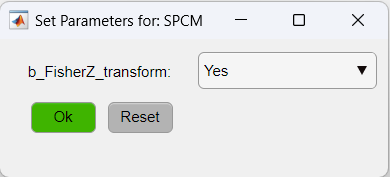
As for the SPCM function, we will apply the Z-Fisher transformation of the correlation data as:

Tip Here, you can save the pipeline with the customized parameters for later use. To do so, just click on the Save button. If you are using the umIToolbox app, the pipeline will be saved in the folder PipelineConfigFiles. To use the saved pipeline, click on the open button.

The pipeline is ready to be applied! Here is a summary of the steps:

run_ImagesClassification: imports the binary data and saves each recording channel in a separate .dat file.
run_HemoCorrection: uses all reflectance channels (i.e. red, green and amber) to subtract the hemodynamic signal from the fluorescence data.
GSR: performs a global signal regression of the fluorescence data to remove global signal variance.
normalizeLPF: performs a temporal band-pass filter between 0.3 and 3Hz and normalizes the data as ΔF/F.
SPCM: Calculates a pixel-based correlation Seed Pixel Correlation Map and applies the Z-Fisher transformation to the correlation values.

Finally, click on the green button Run! to execute the pipeline!

At the end of the execution of the pipeline, a summary table is displayed showing the information of each step of the pipeline. Use this table to spot failed steps and to retrieve error messages for later troubleshooting:

The seed-pixel correlation maps created by the pipeline are stored in the file SPCMap.dat. Click here to learn how to explore the data!